Bulk downloads of space and time targeted MODIS data

First thing you need to get the appropriate software installed, the modis reprojection tool is used by this package to process your data. It can be used outside of R too, but this automates the process.

Then load packages, and set up your login and file path, followed by checking out what modis products are avaialble, and their appropriate codes.

library(raster)

## Loading required package: sp

library(rgeos)

## rgeos version: 0.3-26, (SVN revision 560)
##  GEOS runtime version: 3.4.2-CAPI-1.8.2 r3921 
##  Linking to sp version: 1.2-5 
##  Polygon checking: TRUE

library(rgdal)

## rgdal: version: 1.2-16, (SVN revision 701)
##  Geospatial Data Abstraction Library extensions to R successfully loaded
##  Loaded GDAL runtime: GDAL 2.1.2, released 2016/10/24
##  Path to GDAL shared files: /Users/Maxwell/Library/R/3.3/library/rgdal/gdal
##  GDAL binary built with GEOS: FALSE 
##  Loaded PROJ.4 runtime: Rel. 4.9.1, 04 March 2015, [PJ_VERSION: 491]
##  Path to PROJ.4 shared files: /Users/Maxwell/Library/R/3.3/library/rgdal/proj
##  Linking to sp version: 1.2-5

library(rts) #install and load the rts package for modistools specifically

## Loading required package: xts

## Loading required package: zoo

## 
## Attaching package: 'zoo'

## The following objects are masked from 'package:base':
## 
##     as.Date, as.Date.numeric

## Loading required package: RCurl

## Loading required package: bitops

## rts 1.0-45 (2018-03-17)

#need to set nasa authorization (username and password that are separately acquired online, see link above), but only need to do once with the function below: setNASAauth()
#setNASAauth()
#setMRTpath("/Users/Maxwell/MRT/bin/", update=T) #function to set the path of the modis reprojection tool for the functions to find
#modisProducts() #function to check out possible products (Beware, the version of Modis matters for extracting with ModisDownload later)

#make a date sequence to extract
start<-NULL
end<-NULL
start<-paste0(rep(2016:2018,1) , rep(".01.01",2))
end<-paste0(rep(2016:2018,1),rep(".05.31",2))
start

## [1] "2016.01.01" "2017.01.01" "2018.01.01"

end

## [1] "2016.05.31" "2017.05.31" "2018.05.31"

#combine into one statement for each desired date so it is easy to loop
dateseq<-NULL
dateseq<-paste((start), noquote("\",\""), paste(end), sep = "") 
dateseq

## [1] "2016.01.01\",\"2016.05.31" "2017.01.01\",\"2017.05.31"
## [3] "2018.01.01\",\"2018.05.31"

Now to extract dates we have set up from a particular modis product

#extract dateseq for all of oregon, mosaic, and reproject all in one step using ModisDownload
  ##note the "MOD13A3" is the modis product
    ###h and v are the modis tiles (can look up online which oncs youll need)
      ####bands - each modis product has a bunch of bands, so here can specify which ones you want, need to put 0 or 1 for all or else it may do somethin weird
        #####proj_params Something weird, look up in the package to get a better idea of what to do here.
          ######utm_zone only needed if using UTM
            ######Datum: projection, pixel size: set what you what, mosaic: default is FALSE, need to set to true to mosaic. If you want there is a separate funciton to do it manually. Same                with proj, which reprojects the mosaicked file to a tif. Versopm: important, seems like 006 has everything I wanted, 005 didnt have much.
#download all modis files in the date range to your working directory (set above)

ModisDownload("MOD13A3",h=c(8, 9),v=c(4,4),dates=c("2016.01.01", "2016.05.31"),bands_subset="1 0 0 0 0 0 0", proj_type="UTM",proj_params="0 0 0 0 0 0 0 0 0 0 0 0 0 0 0",utm_zone=c(10,11),datum="WGS84",pixel_size=250, mosaic = T, proj=T, version='006')

## Warning in strptime(x, format, tz = "GMT"): unknown timezone 'zone/tz/
## 2019b.1.0/zoneinfo/America/Los_Angeles'

#Show files of some pattern in WD
listfiles <- list.files(pattern='MOD13') # in wd
listfiles<-listfiles[1:5] #or whatever ones are .tif
plot(raster(listfiles[1])) # take a look at what they look like!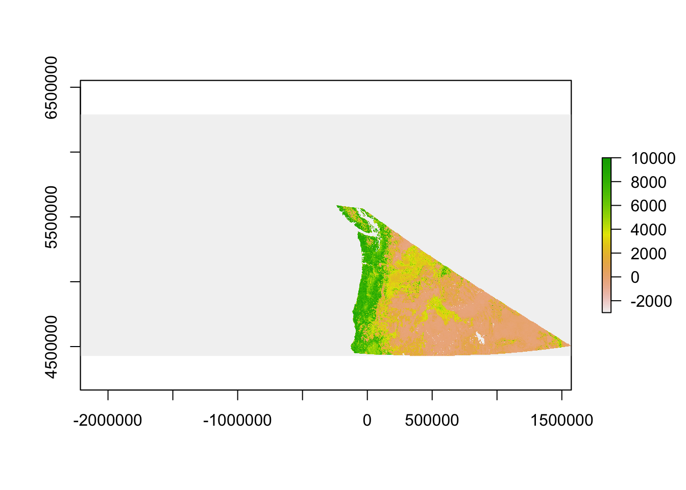

#Download, or get shape files separately if you want to crop, my interest here is Oregon.
oregon<-readOGR(dsn="/Users/Maxwell/Documents/geospatial/orcnty2015/", layer = "orcntypoly")
orutm<-spTransform(oregon, crs(raster(listfiles[1]))) #make sure coordinate systems of shapes and MODIS files match
plot(orutm)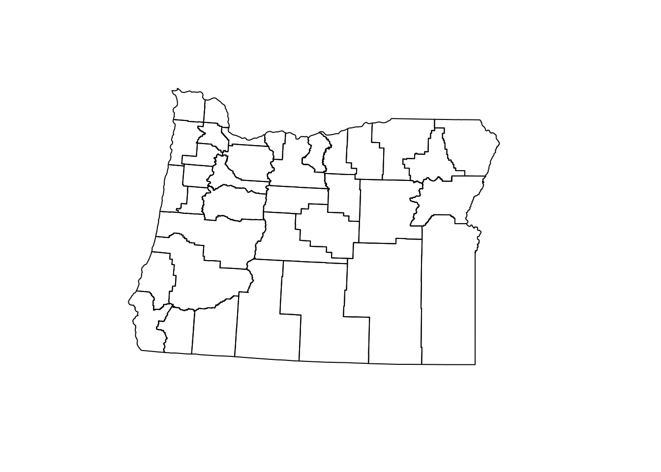

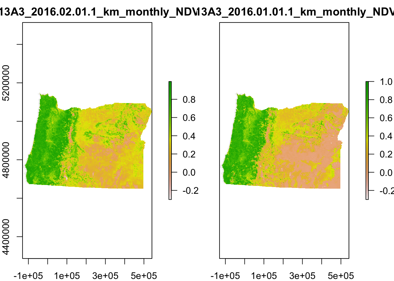
#make a loop to read in all the tif files and crop them to oregon size, then put them all into a rasterstack
r<-NULL
NDVI<-NULL
for(i in listfiles[1:2]) #just doing two of them for demonstration
  {
 r<-raster(i)/10000 #divide by 10000 to get into correct units.
 #extent(r)<-extent(orutm) #match extents
 r<-crop(r, orutm) #crop to size
 r<-mask(r, orutm) #hide outside pixels
 NDVI<-stack(r, NDVI) #put all modified into a single raster stack
}

plot(NDVI)